
How to Use Conditional Formatting in Google Sheets for Common Tasks
Click "Format" in the file menu followed by "Conditional formatting". From the top file menu select Format followed by Conditional formatting . 3. In the "Format cells if" dropdown menu, select "Custom formula is". The Conditional format rules menu will now appear on the right hand side of the display.
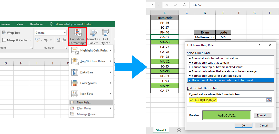
How to Color cell Based on Text Criteria in Excel
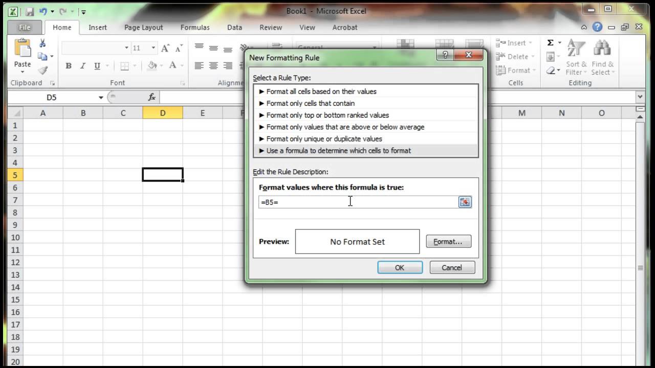
Excel conditional formatting based on another cell value. Excel's predefined conditional formatting, such as Data Bars, Color Scales and Icon Sets, are mainly purposed to format cells based on their own values.If you want to apply conditional formatting based on another cell or format an entire row based on a single cell's value, then you will need to use formulas.
How to conditional formatting based on another sheet in Google sheet?
Rule #1. The following formula will return whether or not the cell is blank. I have selected. =ISBLANK(B2) Note that I have selected cells B2:D5 with relative references. This will apply the same formula changing the cell reference for every cell in the selected range.
How to Clear the Conditional Formatting Rule from Entire Sheet ExcelNotes
Apply Date-Related Conditional Formatting in Google Sheets. Step 1. Step 2. Step 3. Step 4. Step 5. Summary. Conditional formatting is a powerful tool in Google Sheets that can help you visualize your data in a more meaningful way. One way to use conditional formatting is to format cells based on the date in another cell.
Excel Conditional Formatting Based On Another Cell Heelpbook Riset
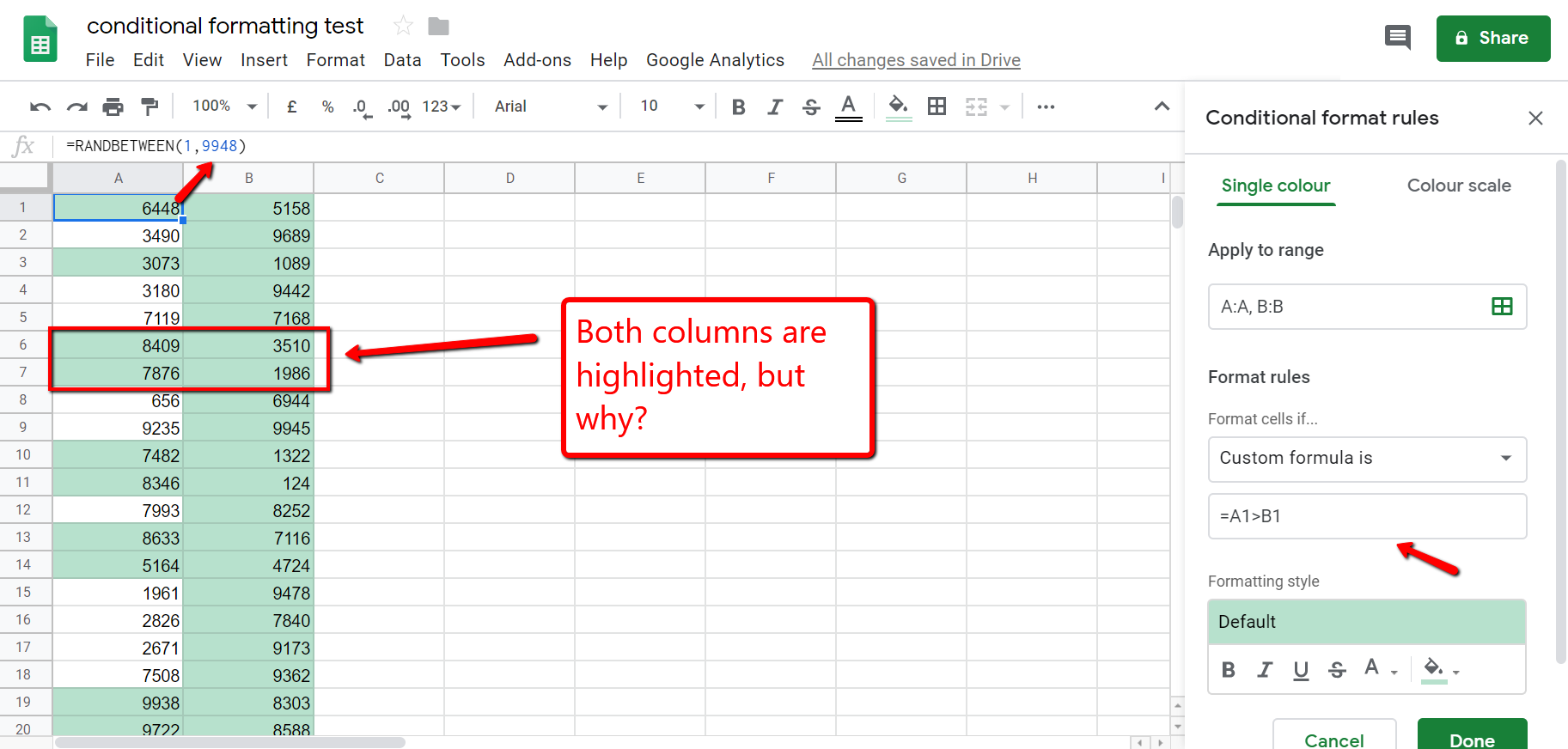
To do so, we can highlight the cells in the range A2:A11, then click the Format tab, then click Conditional formatting: In the Conditional format rules panel that appears on the right side of the screen, click the Format cells if dropdown, then choose Custom formula is, then type in the following formula: Note: It's important that you include.
Conditional Formatting Based on Another Cell YouTube
The process to highlight cells based on another cell in Google Sheets is similar to the process in Excel. Highlight the cells you wish to format, and then click on Format, Conditional Formatting. From the Format Rules section, select Custom Formula. Select the fill style for the cells that meet the criteria. Click Done to apply the rule.
How to Use Conditional Formatting in Google Sheets for Common Tasks
What you can to do is set some column on sheet 1 equal to the appropriate column on sheet 2 (in your example =Sheet2!B6). I used Column F in my example below. Then you can use conditional formatting. Select the cell at Sheet 1, row , column 1 and then go to the conditional formatting menu.
Excel Conditional Formatting Based Another Cell How to Use Advance
Then find the Format menu item and click on Conditional formatting. To begin with, let's consider Google Sheets conditional formatting using a single color. Click Format cells if., select the option "Greater than or equal to" in the drop-down list that you see, and enter "200" in the field below.

Google sheets conditional formatting to colour cell if the same cell in
1. Select the range of cells that you want to apply conditional formatting to. Highlight the cells you want to apply the conditional formatting to. You can click and drag to highlight cells next to each other or select separate cells by holding the Ctrl (Cmd ⌘ on Mac) key when clicking the individual cells.
Conditional Formatting Based on Another Cell in Google Sheets OfficeWheel
Step 5: Set the format style you want. Choose the color or style you want to apply to the cell when the condition is met. After you have set up the conditional formatting based on another cell, you'll notice that the cell's appearance changes automatically when the value in the referenced cell changes. This gives you instant visual feedback.

Conditional Formatting In Excel Explanation And Examples Ionos Riset
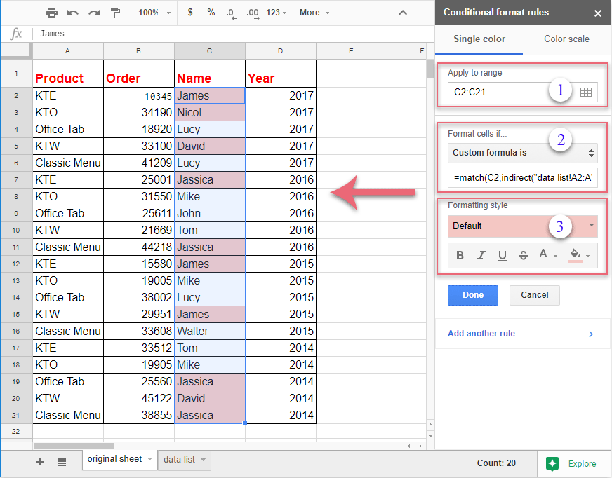
One way to use conditional formatting is to format cells based on the values in another sheet. This can be helpful if you have a large spreadsheet with multiple sheets, and you want to quickly see which cells meet certain criteria. We can use the INDIRECT function in our custom formula to return values from references outside the current sheet.
How to Use Conditional Formatting to Automatically Format Cells Based
Color scales in Google Sheets let you format different cells with different colors based on the cells' values. Unlike single-color conditional formatting, which allows you to define your own colors, Google Sheets assigns a predefined color to the lowest value, another predefined color to the highest value, and a weighted blend of the two to.
Excel Conditional Formatting one cell based on another cell's value
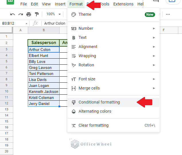
Step 2: Go to Format > Conditional formatting. Here's another easy step. Simply move your cursor to the Google Sheets Menu section and select the Format option. This action will reveal all of the Format menu items, including Conditional formatting. Simply click on it to open it in the right-hand pane.
Conditional Formatting Based on Another Cell in Google Sheets OfficeWheel
Here's how to use Google Sheets conditional formatting if another cell contains text: Step 1: Select the cells that you want to highlight (student's marks in this example) Step 2: Click the Format option. Step 3: Click on Conditional Formatting. This will open the Conditional Formatting pane on the right.
Use name in custom formatting excel boutiquepilot
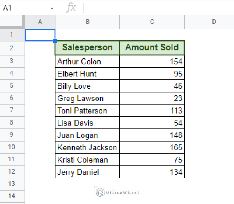
The conditional formatting functionality comes to the rescue, with which you can change the cell colors based on the cell value in Google Sheets. To apply this formatting, first select all the cells in column B. Now navigate to Format > Conditional formatting. A sidebar opens up on the right side of the screen.
Spreadsheet conditional formatting definition emporiumsenturin
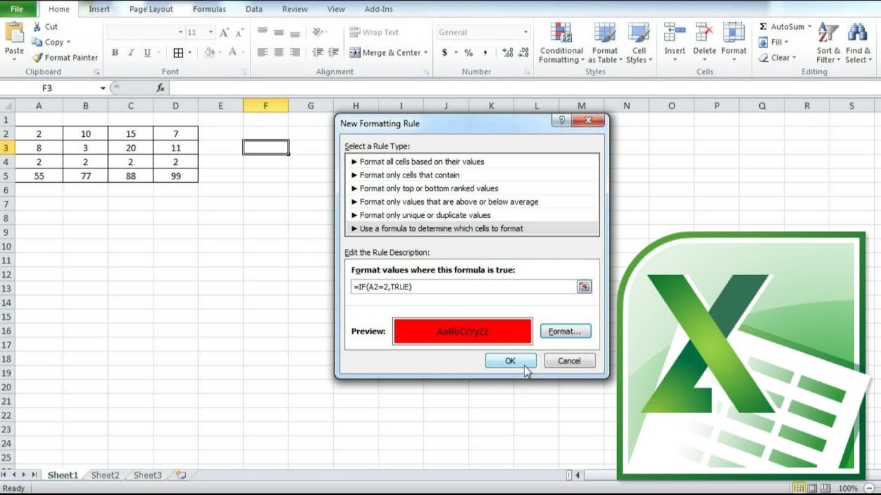
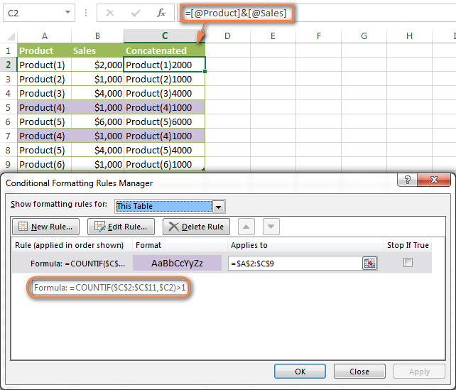
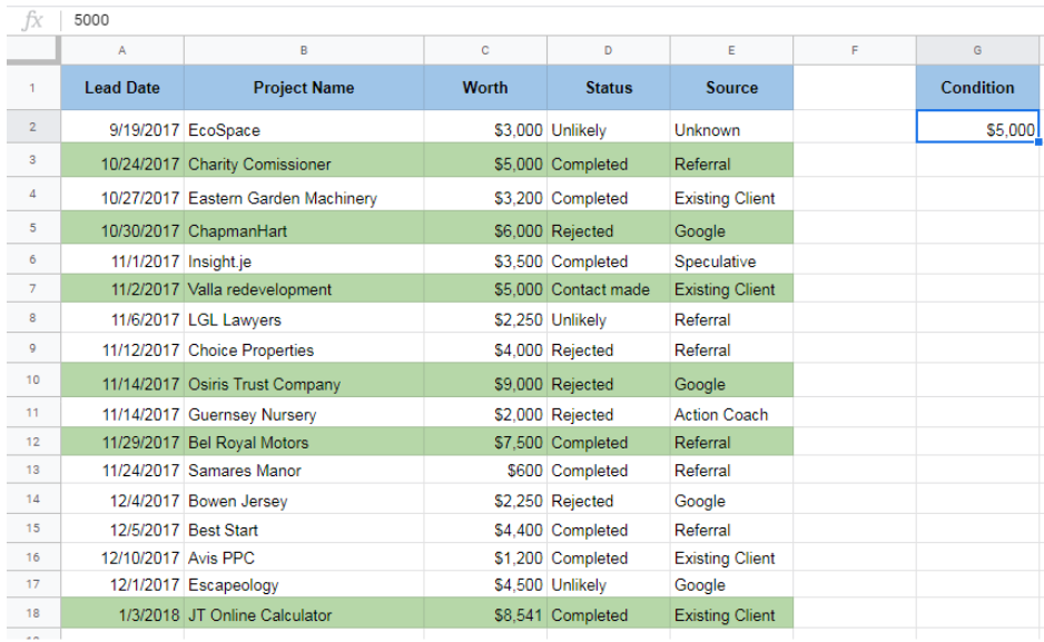
To apply conditional formatting based on a value in another cell, you can create a rule based on a simple formula. In the example shown, the formula used to apply conditional formatting to the range C5:G15 is:
- Caldera Baxiroca Victoria Plus 24 24f Errores
- Cuando Meten Esmeralda En El Lol
- Ciclos Superiores Nutricion Y Dietetica Vigo
- Como Solicitar Documentacion En Industria De Alava
- How Much Money Can You Withdraw From An Atm
- Monasterio Del Escorial Balas De Cañon Y Parrillas
- Honda Africa Twin Garmin Travel Edition
- Mueble Auxiliar Cerezo 50 45 X 73
- Casa En El Arbol Extremadura
- Is Toyota Still Replacing Tacoma Frames